Fix a target
Choose a class logit, or a fixed annotated region for segmentation. The target must not change when inputs are masked.
Which spectral channels matter, and where?
SSI attributes a model score to individual spatial cells and input channels. It keeps the surrounding image observed while measuring how channels within one cell contribute to the selected prediction.
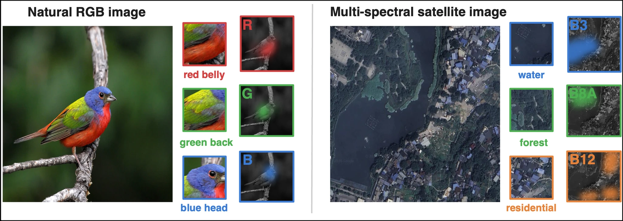
A spatial map identifies relevant locations. A channel ranking summarizes relevance across an image. Neither alone tells us whether the same channel matters differently at different positions.


Rather than enforce a rank-one product of one spatial map and one spectral vector, SSI retains a joint matrix of cell-by-channel contributions. Those contributions can be positive or negative.
For a selected spatial cell, SSI measures the effect of its channels while the entire external image remains observed. Shapley values allocate that cell's masking contrast among its channels.
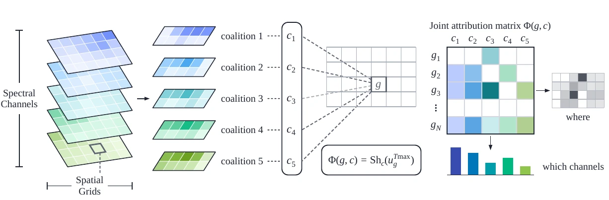
The highlighted cell is the only cell whose channels may be masked; all others remain observed.
Evaluate the chosen channel's marginal contribution across channel coalitions within this cell.
Choose a class logit, or a fixed annotated region for segmentation. The target must not change when inputs are masked.
Only channels in cell g are changed. Masked values use a specified per-channel baseline.
Use ordinary Shapley values over the local channel game. Sum by cell or channel for two marginal summaries.
Exactly true for the local Shapley game (up to numerical or permutation-sampling error). It does not imply global input-to-baseline completeness after summing across cells.
The observed-context construction differs from MC-Owen attribution, which averages over external spatial coalitions. Read the paper for formal definitions and experimental assumptions.
This is an actual repository example. The preview is a stored high-resolution research figure. Use the live Playground to recompute SSI from the original six-band tensor and verified ONNX checkpoint.
 PUBLISHED ATLAS FIGURE · NOT A LIVE RUN
The fixed target is the annotated burn region. A signed spatial map is the sum over all six channels; per-channel overlays and the spectral summary preserve channel identities.
Primary preview loads directly from the SSI repository; if unavailable, the image switches to labeled paper Figure 4, not a replacement sample result.
Compute this example ↗If your browser blocks embedded frames, open the Playground directly. Live calculation occurs in that application.
Results below are transcribed from the NeurIPS paper, not produced by this web page. Error bars show reported bootstrap standard deviations, not confidence intervals or significance tests.
Mean intersection-over-union of top-ranked spatial cells with the dataset's spatial annotation proxy.
TABLES 8–9 · mIoU ↑Hit@K measures recovery of a predefined class-specific positive-prior band set; it is not pixel-level attribution ground truth.
TABLES 10–11 · Hit@K ↑The reported evaluation counts were up to 4,480 for SSI and 76,800 for MC-Owen. These are forward-pass counts, not wall-clock speed measurements.
SSI evaluations relative to MC-Owen
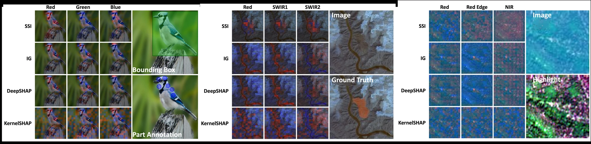
Browse the complete released gallery across six model families. CUB-200, EuroSAT and HLS are in the paper's main benchmarks; PaviaU, Salinas and WHU-Hi-LongKou are additional interactive examples.
The core public API accepts a model, a model-ready multichannel tensor, a fixed target, and a numerical per-channel baseline.
from ssi import SSI

result = SSI(
    model=my_model,
    input=my_image,                # model-ready CHW tensor
    target=6,                      # fixed output class
    baseline=dataset_channel_mean,# one numeric value per channel
    image_size=(128, 128),
    grid_size=16,                  # cell extent in pixels -> 8x8 cells
    permutations=5,
).explain()

spatial, spectral = result.spatial, result.spectralAPI grid_size refers to cell extent in pixels. The paper's 8×8 or 16×16 grid refers to the number of cells along each axis. Segmentation requires a fixed target region; a displayed RGB preview cannot replace the original multispectral input tensor.
External cells remain observed. SSI's within-cell allocation does not claim global completeness across interacting spatial locations.
Attributions depend on the model, target definition and specified masking baseline. Negative contributions are meaningful.
More bands increase the cost of local coalition evaluation; grouping and selective evaluation can be useful future directions.
Haotian Ma, Ruqi Yang, and Philip Townsend. Spectral-Spatial Interpretation. NeurIPS 2026. arXiv:2610.21114.
Figures and numerical results reflect the SSI paper and public repository. HLS derived data retain CC-BY-4.0 attribution. Other paper figures, weights and third-party source code may have distinct licenses.
Third-party notices ↗